Excel dashboards transform raw data into clear, actionable visuals, making spreadsheets intuitive and impactful. They distill key insights, helping you or your team focus on what matters most—whether tracking personal projects or business metrics.
As an Excel power user with years of experience building dashboards for reports and trackers, I'll walk you through creating one for my annual review of The Simpsons Treehouse of Horror episodes. These proven techniques scale to sales pipelines, fitness logs, or any dataset.
Master these three techniques to craft efficient, visually appealing dashboards. Keep data calculations on hidden sheets for a clutter-free main view—always verify document settings before sharing.
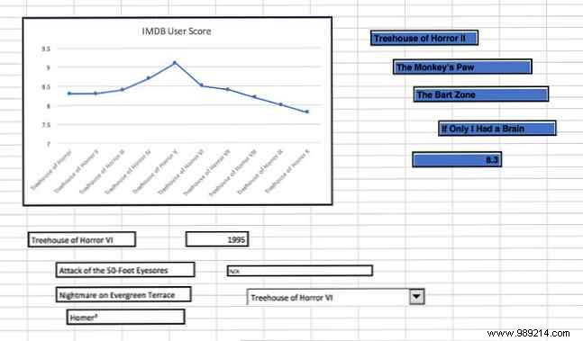
The Camera tool captures any spreadsheet range as a live image, perfect for dynamic charts on your dashboard.
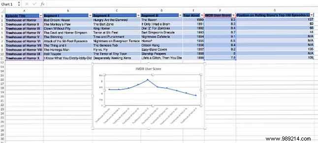
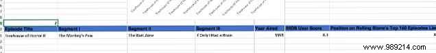
Start with a simple data table tracking IMDb ratings for episodes.
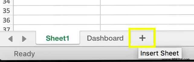
Create a new sheet named Dashboard.
Select your chart range, click the Camera tool (add to Quick Access Toolbar if missing via File > Options > Quick Access Toolbar > Camera), then paste into the Dashboard sheet.
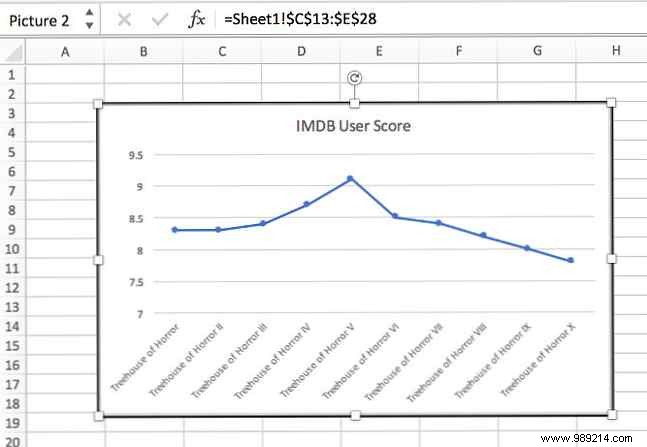
Position roughly for now; refine the design later.
Dropdown menus let users switch data instantly, keeping dashboards focused and interactive.
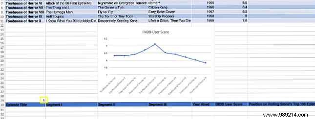
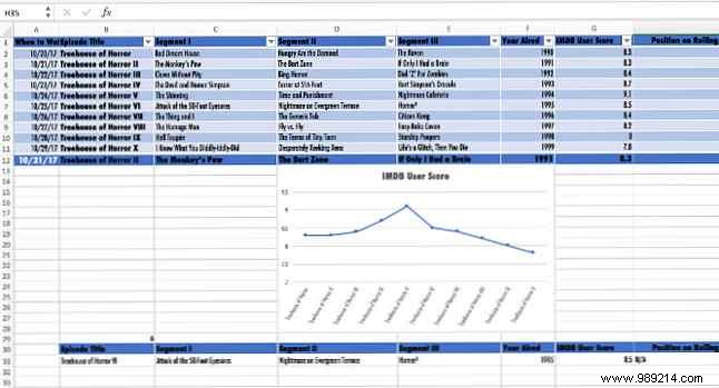
In your data sheet, duplicate headers lower down and add a yellow-highlighted placeholder cell (e.g., A29) starting at 1.
In the cell left of the pasted table, enter:
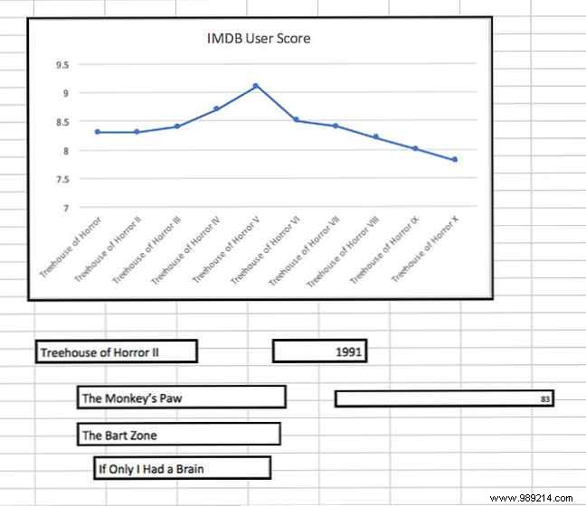
=INDEX(A2:G11, $A$29, 0)Adjust ranges to match: first covers data body, second is the placeholder (absolute reference), third is 0 for full row.
Drag across the row.
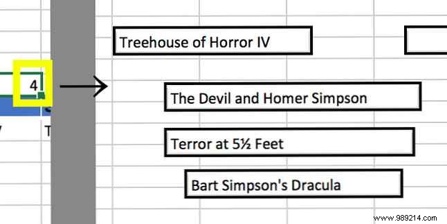
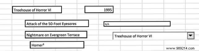
Updating the placeholder (e.g., to 2) pulls the corresponding row— the foundation for your dropdown.
Use Camera to snapshot a data cell and place on Dashboard.
Test by changing the placeholder manually.
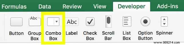
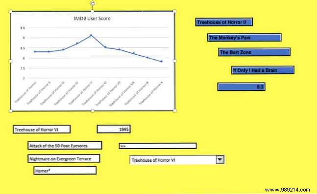
Enable Developer tab (File > Options > Customize Ribbon). Insert a Combo Box (Form Control).
Right-click > Format Control: Set Input Range to your list (e.g., episode numbers), Cell Link to the placeholder (e.g., $A$29). Use sheet references if needed.
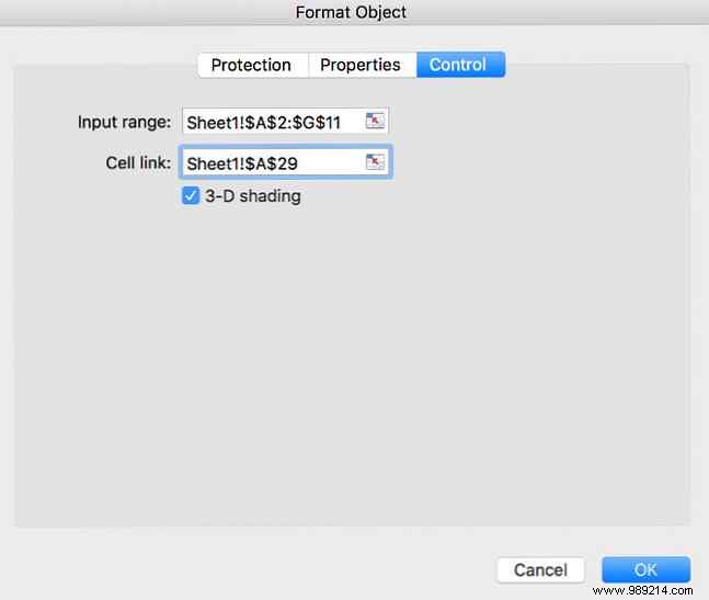
Test the dropdown—it drives live updates.
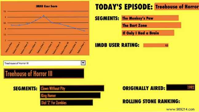
Automate daily priorities with date-driven lookups.
Add a date column to your data sheet for watch dates (or task due dates).
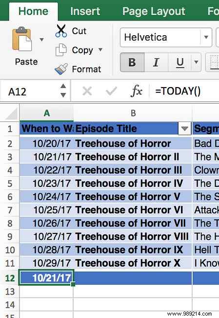
Below, use =TODAY() for current date. Right of it:
=VLOOKUP(A12, A2:B11, 2, FALSE)A12 is today; range is date:episode; 2 returns episode column; FALSE for exact match.
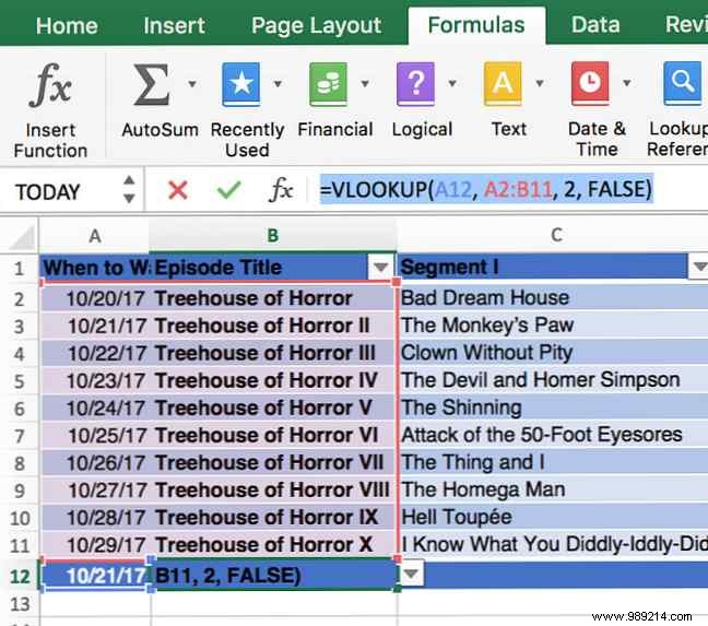
Fill row and Camera it to Dashboard.
Finalize with bold fonts, high contrast, and thematic colors for at-a-glance readability. Hide gridlines (Page Layout > Sheet Options > uncheck Gridlines > Print). Format cells for backgrounds (e.g., Simpsons yellow).
Adjust source cells: Futura font, black/orange scheme, narrow numeric widths.
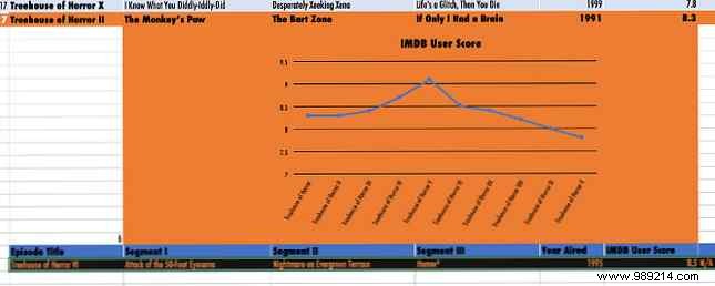
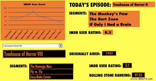
Your dashboard now updates via date and dropdown—clear, concise, informative.
Adapt these for task lists or reports: pair TODAY() with formulas for scheduling, Camera for flexibility. Excel's power lies in matching tools to goals.
What's your favorite Excel dashboard trick? Share in the comments!