It's two days before your tax deadline. You've got a box full of receipts, pay stubs, bills, and forms—and you can't afford another late fee. What now?
Skip the costly emergency accountant visit. Instead, leverage Excel's powerful formulas to organize everything quickly and accurately. As an experienced Excel user who's helped countless filers, I've relied on these five formulas for years to streamline tax prep.
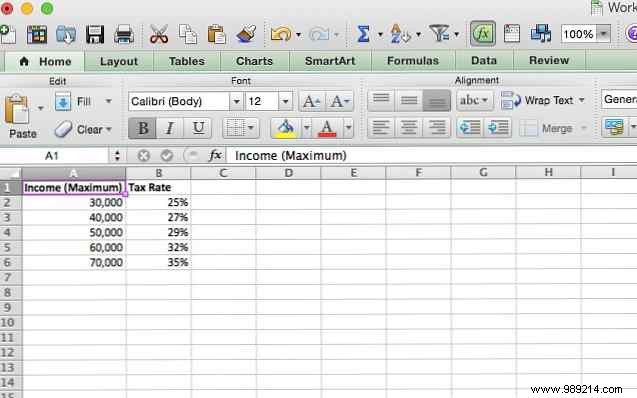
VLOOKUP shines for tax brackets. Set the range_lookup to TRUE, and it returns the largest value less than or equal to your lookup value—ideal for progressive rates.
Here's a sample tax table:
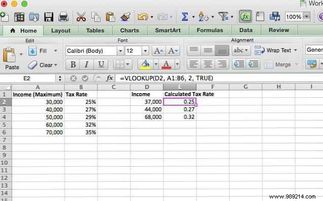
For incomes of $37,000, $44,000, and $68,000, use this formula:
=VLOOKUP(A2, A1:B6, 2, TRUE)
A2 is income; A1:B6 is the table range; 2 returns the tax rate column; TRUE approximates downward. Results:
Multiply the rate by income for tax owed. Note: Tables must use upper bracket limits for accurate rounding down. For advanced tips, see Ryan's guide on 3 Crazy Excel Formulas That Do Amazing Things.
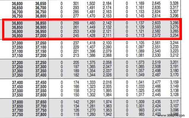
Tax credits like the Earned Income Credit (EIC) vary by income thresholds. Nest IF with AND for precise checks.
Sample EIC table (single filers highlighted):
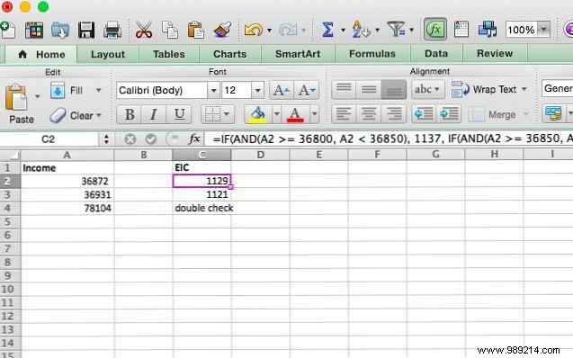
Formula example:
=IF(AND(A2>=36800, A2<36850), 1137, IF(AND(A2>=36850, A2<36900), 1129, IF(AND(A2>=36900, A2<36950), 1121, IF(AND(A2>=36950, A2<37000), 1113, "double check"))))
Each IF tests a range; unmatched values prompt "double check." In action:
VLOOKUP can substitute here too. Learn more Boolean logic in our Excel Mini Tutorial or build templates from our 15 Useful Spreadsheet Templates.
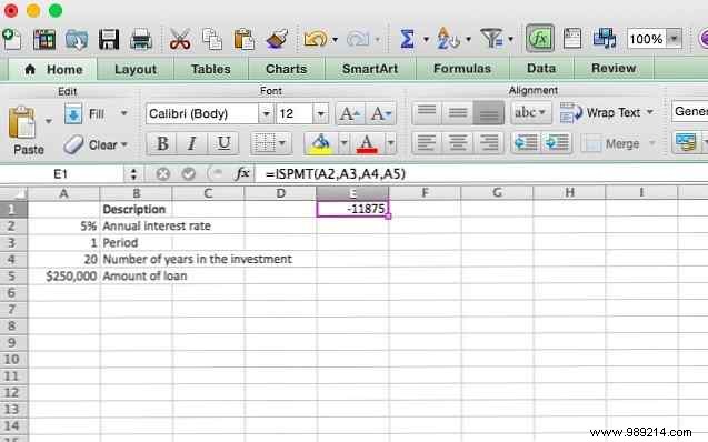
Calculate deductible loan interest if your lender doesn't provide Form 1098. Use IPMT:
=IPMT(rate, period, nper, pv)
Rate is per-period interest; period is current (e.g., 1 for year 1); nper is total periods; pv is loan amount.
For a $250,000 mortgage at 5% over 20 years (annual):
=IPMT(0.05, 1, 20*12, 250000)
Adjust for monthly: divide rate by 12, use months. Sample table:
Uncover true loan costs from nominal rates compounded multiple times yearly:
=EFFECT(nominal_rate, npery)
Example: 7.5% nominal, quarterly compounding:
=EFFECT(0.075, 4)
Returns 7.71% effective APR. Pair with budgets via our Personal Budget in Excel guide.
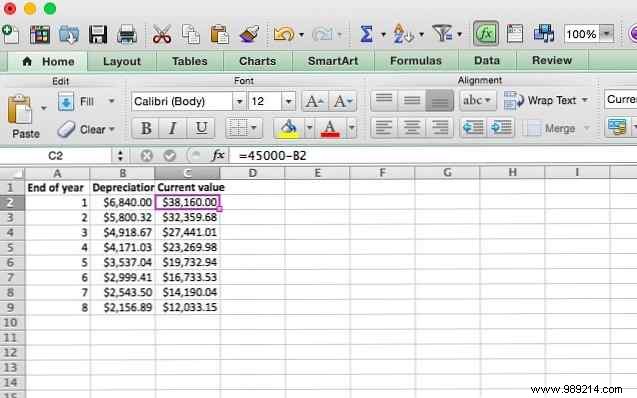
For fixed-declining balance depreciation:
=DB(cost, salvage, life, period)
$45,000 asset to $12,000 salvage over 8 years:
=DB(45000, 12000, 8, 1)
Repeat for periods 1-8; subtract from prior book value annually:
These formulas kickstart your tax workflow. Not an Excel pro? Try Google Drive tools in our 10 Money Management Tools or IRS resources via 7 IRS Website Tools and free templates from top sites.
Share your go-to Excel tax tips below! What formulas save you time? Ask questions—we're here to help.