3 Advanced Excel Formulas to Supercharge Your Spreadsheets

Microsoft Excel remains a powerhouse for data analysis and automation, packed with formulas and features that can transform raw data into actionable insights. As an Excel expert with over a decade of experience optimizing workflows for businesses, I'll share three advanced techniques using formulas and conditional formatting to elevate your skills.

Unlocking Excel's Hidden Potential

We've explored Excel for everything from custom calendars to project trackers. The real magic happens with formulas that dynamically manipulate data, adapting seamlessly to new inputs.

Let's explore practical examples to harness these capabilities effectively.

Conditional Formatting with Formulas for Dashboard Magic

Conditional formatting is underutilized but incredibly powerful. For deeper dives, check Sandy's expert guide on formatting data in Excel with conditional formatting.

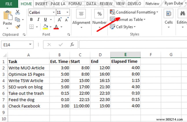
Combined with formulas, it turns spreadsheets into interactive dashboards. Access it via Home > Conditional Formatting.

Options abound for highlighting cells based on values, like color-coding with IF statements. Learn more about IF functions in Excel.

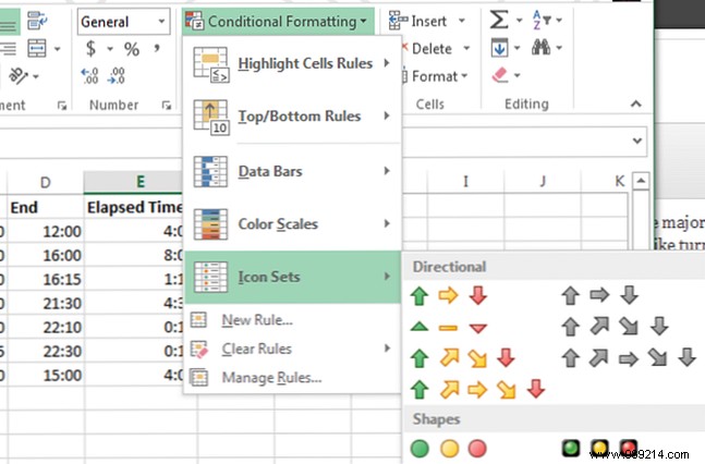
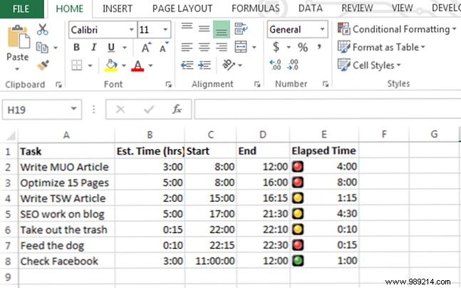
Icon Sets stand out for visual dashboards. Here's a selection:

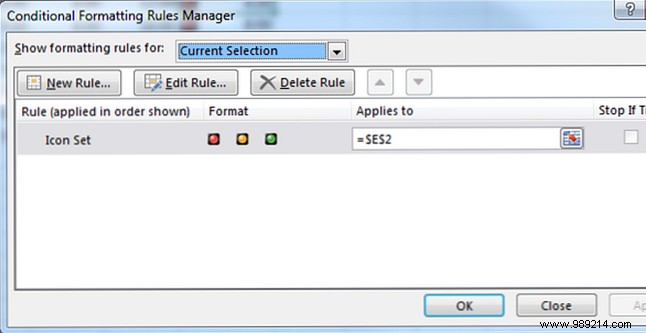
Click Manage Rules to open the Rules Manager.

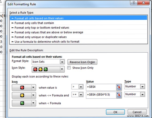
Edit rules to customize logic. In this example, track task time against budgets: yellow at 50%, red when exceeded.

The dashboard reveals overruns:

Time to refine your schedule!

1. Reverse VLOOKUP with CHOOSE

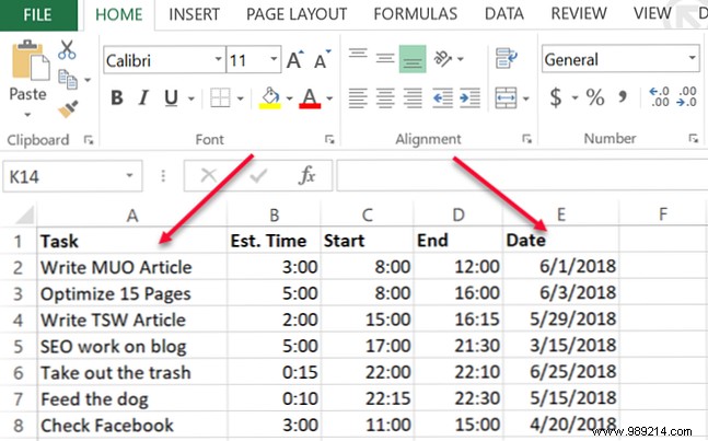
VLOOKUP is a staple, but it requires lookup values on the left. What if you need the reverse?

For this dataset, find the task for 6/25/2018:

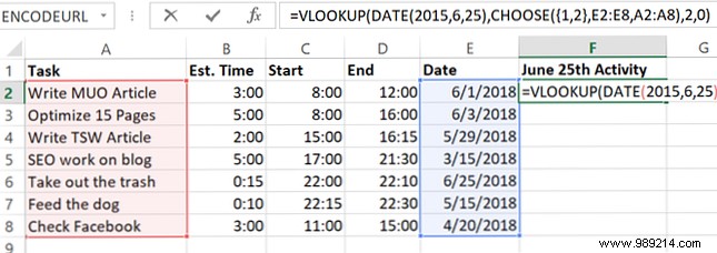
Standard VLOOKUP won't work left-to-right. Forums suggest INDEX/MATCH, but nest CHOOSE inside VLOOKUP instead:

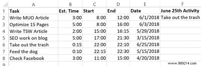
=VLOOKUP(DATE(2018,6,25),CHOOSE({1,2},E2:E8,A2:A8),2,0)

This reorders columns virtually: dates as index 1, tasks as 2. Result:

Reverse lookup achieved! For more, see Dann's article on finding data in Excel.

2. Nested Formulas to Parse Delimited Strings

Importing delimited data? Parse it without tools. Example: "Ryan; 123 Main St; Portland, ME 04076".

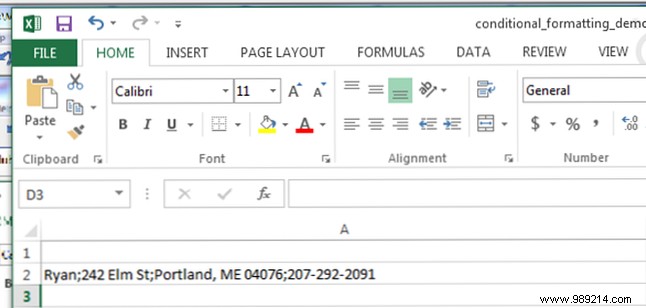
For the name (first field):

=LEFT(A2,FIND("; ",A2,1)-1)

Logic:

• FIND the delimiter in A2
• Subtract 1 for end position
• LEFT extracts up to there

Outputs "Ryan".

3. Deeply Nested Parsing for Subsequent Fields

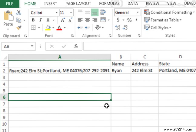
For middle fields, nest RIGHT and LEFT. Street number example:

=LEFT(RIGHT(A2,LEN(A2)-FIND("; ",A2)),FIND("; ",RIGHT(A2,LEN(A2)-FIND("; ",A2)),1)-1)

Build iteratively: RIGHT peels off left parts, then LEFT grabs the next segment.

For the final field, nest further:

=LEFT(RIGHT(RIGHT(A2,LEN(A2)-FIND("; ",A2)),LEN(RIGHT(A2,LEN(A2)-FIND("; ",A2)))-FIND("; ",RIGHT(A2,LEN(A2)-FIND("; ",A2)))),FIND("; ",RIGHT(RIGHT(A2,LEN(A2)-FIND("; ",A2)),LEN(RIGHT(A2,LEN(A2)-FIND("; ",A2)))-FIND("; ",RIGHT(A2,LEN(A2)-FIND("; ",A2))))),1)-1)

Extracts "Portland, ME 04076".

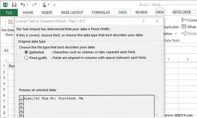
Impressive, but simpler: Data > Text to Columns.

Master Excel's Full Power

These formulas showcase Excel's depth, but simplicity often wins. Start with our Beginner's Guide to Microsoft Excel to build productivity from the ground up.