How to Create a Dropdown List in Excel: Complete Step-by-Step Guide

Dropdown lists in Excel streamline data entry by restricting inputs to predefined options, minimizing errors like typos or inconsistencies. As an Excel expert with years of experience building forms and data tools, I've relied on these features for efficient spreadsheets. Whether for surveys, inventories, or reports, mastering dropdowns boosts productivity.

How to Create a Dropdown List in Excel

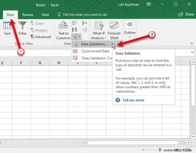
Follow these proven steps to set up a custom dropdown:

1. Create a named range: List your options in cells (column or row), select them, type a name in the Name Box, and press Enter.
2. Add data validation: Select the target cell, go to Data > Data Validation.
3. Link the named range: In Settings, choose List, enter =YourRangeName (e.g., =Food) in Source, and click OK.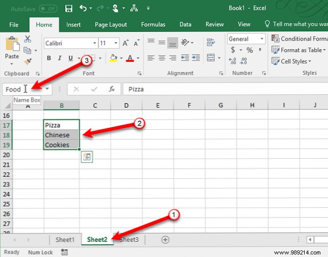
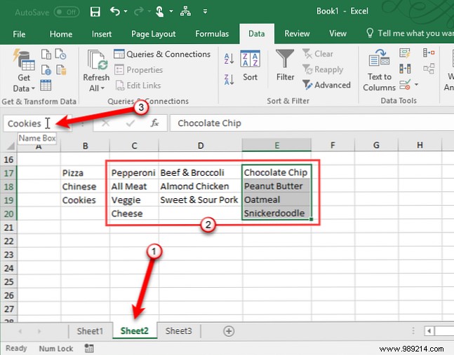
4. Optional: Set input message: Switch to Input Message tab, check 'Show input message...', add title and text for user guidance.

1. Create a Named Range

On Sheet2, enter items like food types (e.g., Pizza, Chinese, Cookies) in cells. Select them, name the range 'Food' in the Name Box.

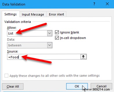
Leave 'Ignore blank' checked to allow empty cells, or uncheck to require selection.

2. Customize Input and Error Messages

In Data Validation, go to Input Message tab: Check 'Show...', add title/message. For errors, use Error Alert tab: Select style (e.g., Stop), add title/message.

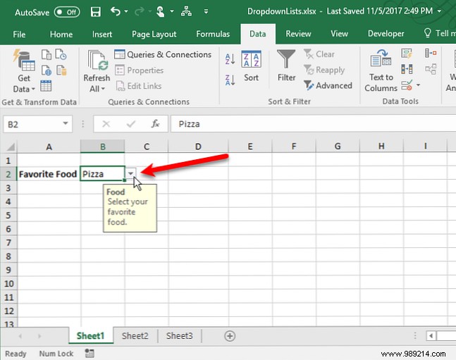
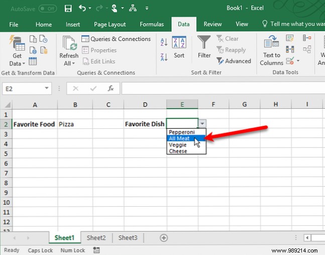
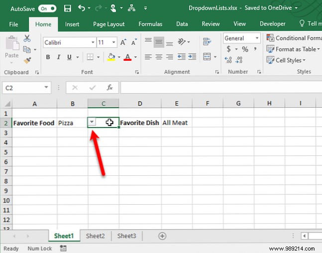
Clicking the cell shows a tooltip; arrow appears on selection. Lists over 8 items get scrollbars.

Advanced Dropdown Options

Edit or Delete a Named Range

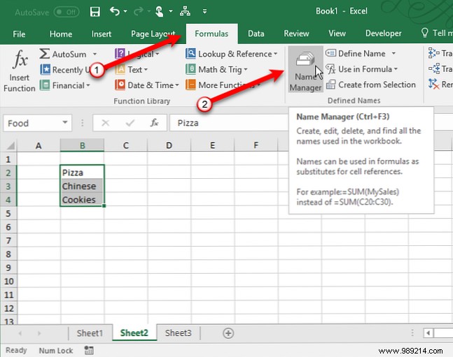
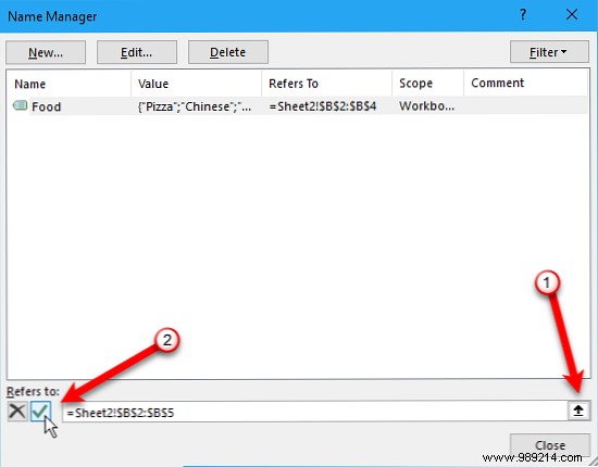
Go to Formulas > Name Manager. Select name, edit range via button or Edit dialog, or Delete.

Create Dependent Dropdowns

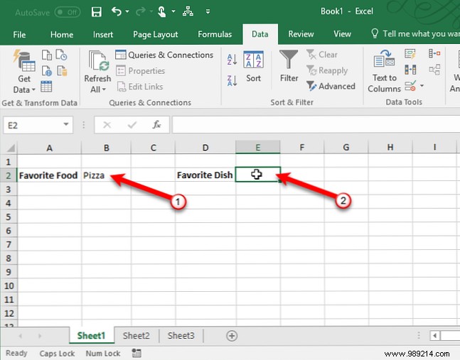
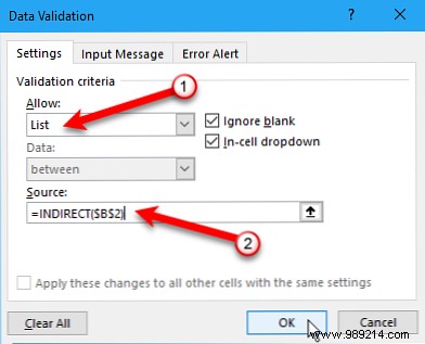
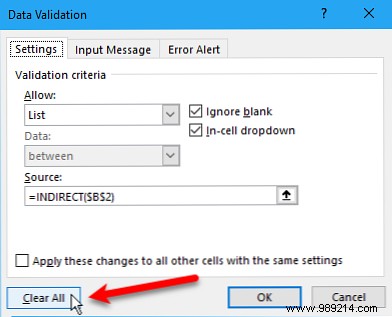
For cascading lists: Name sub-lists matching main options (e.g., 'Pizza', 'Chinese'). In dependent cell's Data Validation (List), use Source: =INDIRECT($B$2) (adjust cell ref).

Copy Dropdowns

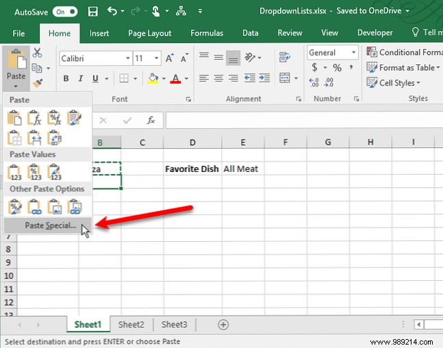
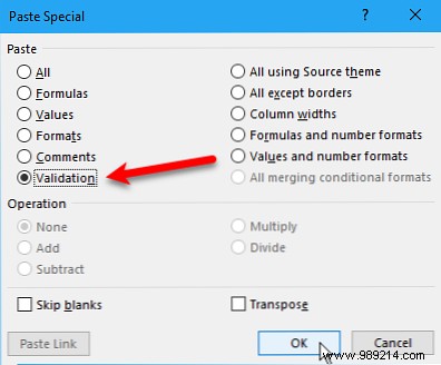
Copy cell (Ctrl+C), Paste Special > Validation only to duplicate rules without formatting.

Note: Pasting over a dropdown erases it—use Ctrl+Z to undo.

Select All Dropdown Cells

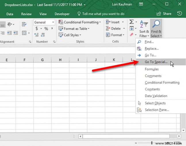
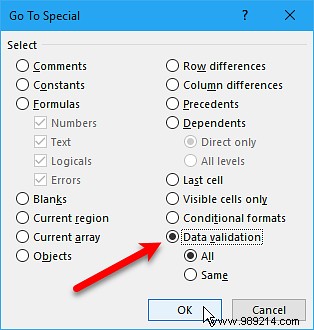
Select one, Home > Find & Select > Go To Special > Data validation > All.

Make Dropdown Arrow Always Visible

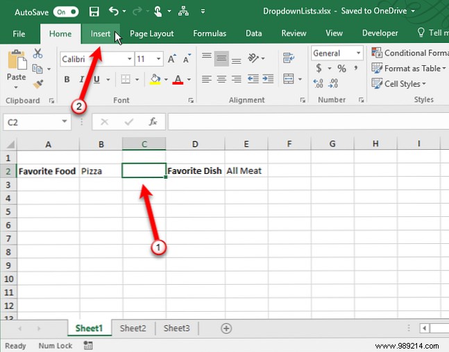
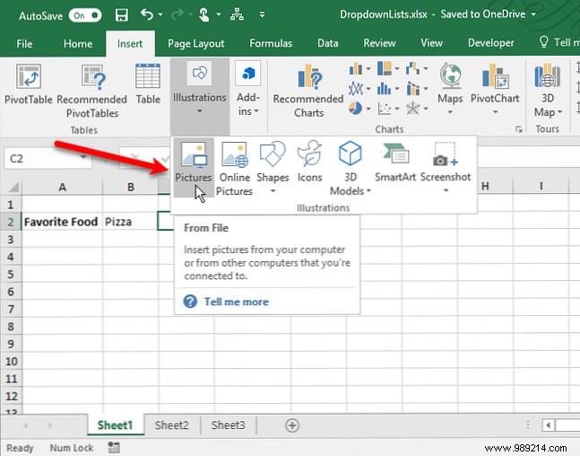
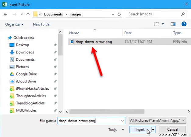
Insert a dropdown arrow image next to the cell: Download drop-down-arrow.png, Insert > Pictures.

Remove a Dropdown

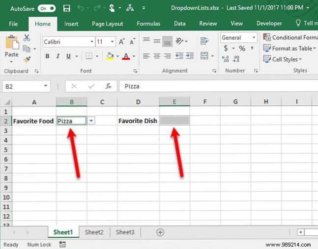
Select cell, Data Validation > Clear All > OK. Cell retains value; paste blank to clear.

Maximize Dropdowns in Your Work

These tools transform data entry—experiment with Developer tab form controls too. How do you use dropdowns? Share below.