As a seasoned Excel expert with over a decade of experience helping professionals streamline their workflows, I know how overwhelming large spreadsheets can be. Hiding and unhiding rows and columns is a simple yet powerful way to focus on the data that matters most. Here's how to do it efficiently.
How to Hide Columns and Rows in Excel
- Select the column(s) or row(s) you want to hide. For contiguous selections, hold Shift; for non-contiguous, use Ctrl (or Command on Mac).
- Alternatively, enter the row or column identifier (e.g., '2:2' for row 2) in the Name Box to the left of the formula bar.
- With your selection active:
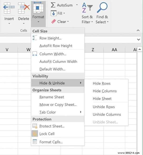
- On the Home tab, in the Cells group, click Format > Hide & Unhide > Hide Rows or Hide Columns.
- Or right-click the selected column or row header and choose Hide. (Note: This won't work if using the Name Box method.)
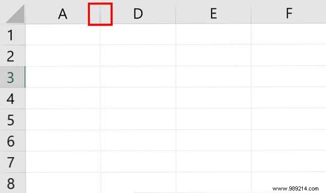
- The hidden row or column disappears, replaced by a thin double line indicating its position.
How to Unhide Columns or Rows
Select the hidden rows or columns using these methods:
- Right-click the thin double line and select Unhide.
- Click the double line to highlight the boundary, or press Ctrl+A (Command+A on Mac) to select all. Then, on the Home tab, go to Format > Hide & Unhide > Unhide Rows or Unhide Columns.
You can hide or unhide multiple rows or columns at once, but not rows and columns simultaneously.
What's your go-to Excel productivity hack? Share in the comments below!