As seasoned Excel professionals with years of experience optimizing spreadsheets for businesses and analysts, we've mastered techniques to declutter worksheets. Whether dealing with dense data or small screens, hiding elements streamlines visibility and analysis without losing functionality.
In this guide, we'll walk you through proven methods to hide and show overflow text, comments, cell contents, formulas, the formula bar, rows, and columns—preserving all data integrity.
When text exceeds a cell's width, it spills into adjacent cells. If those cells contain data, the overflow is truncated. Wrapping text works but expands row height. To hide overflow entirely—even in empty adjacent cells—follow these steps:
Select the cell with overflowing text, then:
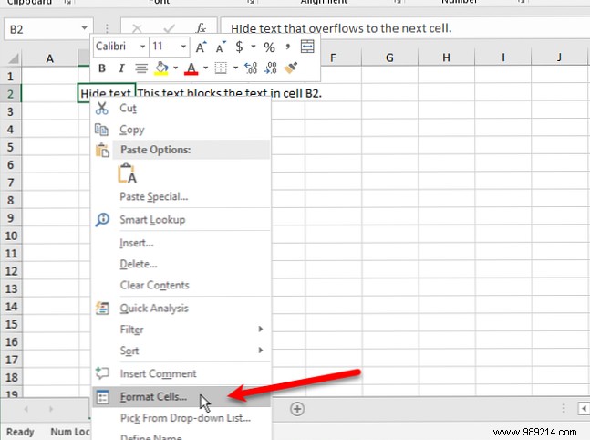
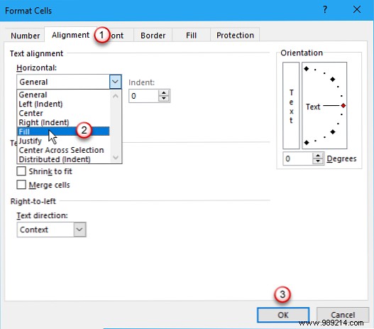
In the Format Cells dialog, go to the Alignment tab. Under Horizontal, select Fill and click OK.
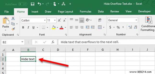
The overflow now stays hidden, keeping your sheet clean. For more on text handling, check our tips for Excel text functions.
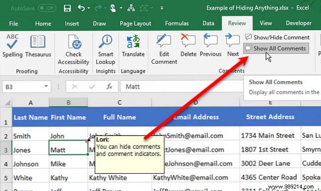
Excel comments are ideal for collaboration, notes, or formula explanations. With many comments, though, they clutter the view. By default, commented cells show a red triangle indicator.
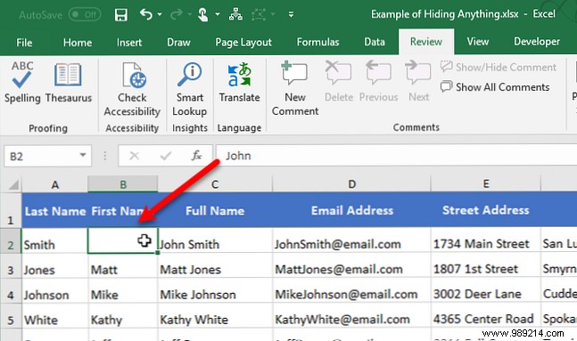
To hide a single comment: Select the cell and either right-click to select Show/Hide Comment or use the Review tab's Comments group.
Toggle multiple with Ctrl selections. To show all: Click Show All Comments on the Review tab—it affects all open workbooks.
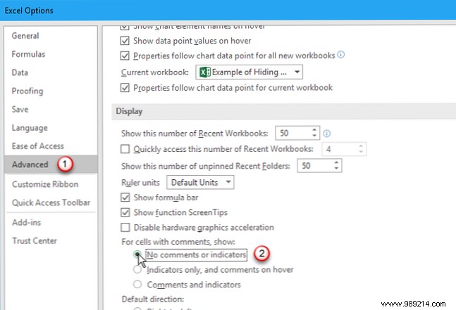
To hide comments and indicators globally: Go to File > Options > Advanced, scroll to Display, and select No comments or indicators under For cells with comments, show. Hovering won't trigger popups.
Reverse by choosing another option or Show All Comments. These settings sync across Excel Options and the Review tab. See our comments guide for details.
You can't hide cells outright, but conceal their contents while keeping them functional for formulas.
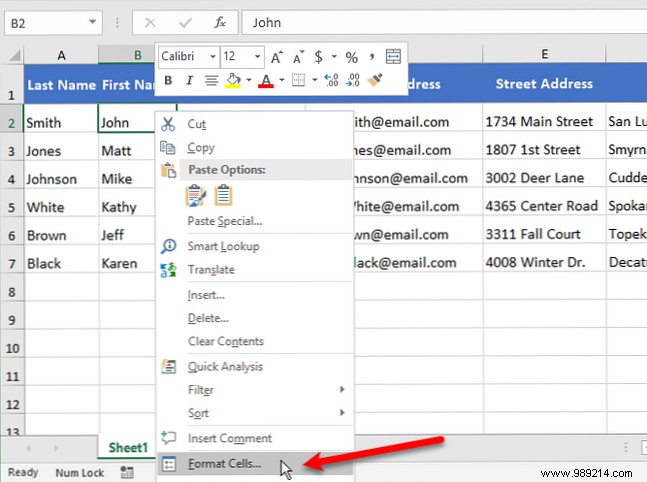
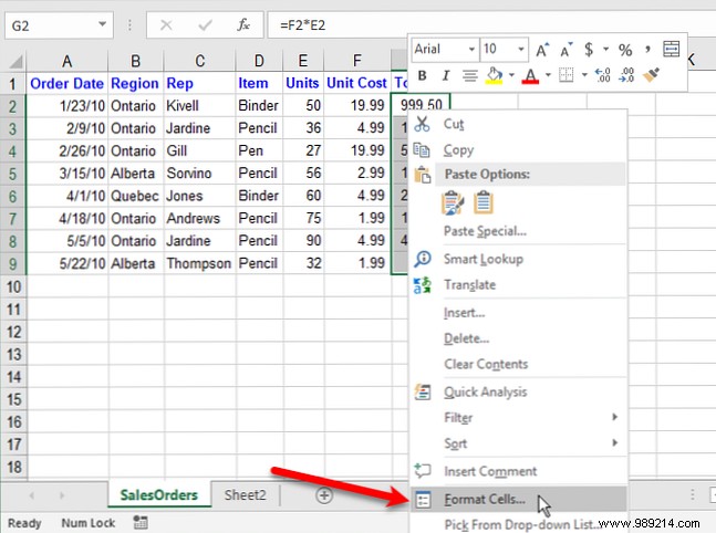
Select cells (use Shift/Ctrl for multiples), then right-click Format Cells or Ctrl + 1.
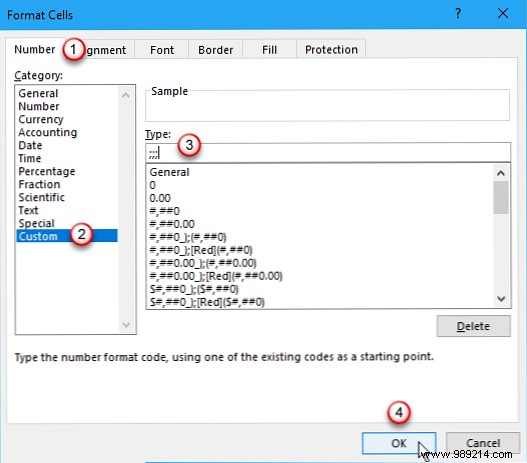
On the Number tab, choose Custom. Note the current Type for reversal. Enter ;;; (three semicolons) and click OK.
Contents vanish but appear in the formula bar and work in calculations. Restore by reselecting Custom and original Type.
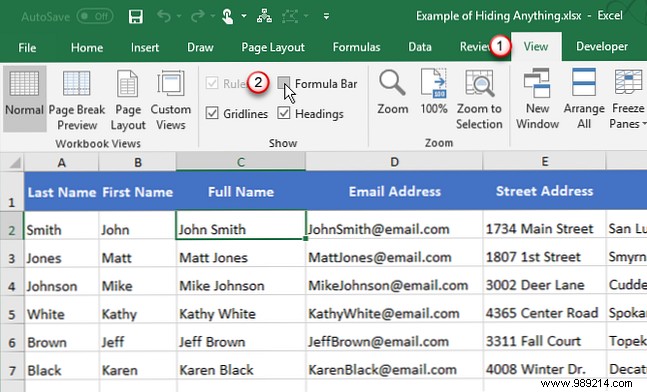
Hidden cell contents still show here. Hide it via View tab: Uncheck Formula Bar in Show.
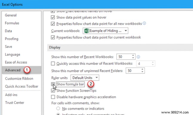
Or File > Options > Advanced, uncheck Show Formula Bar in Display.
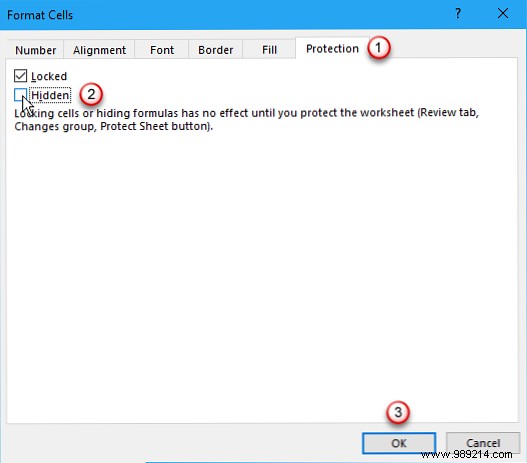
Hide formulas securely by marking cells Hidden and protecting the sheet. First, select cells, Format Cells > Protection tab, check Hidden.

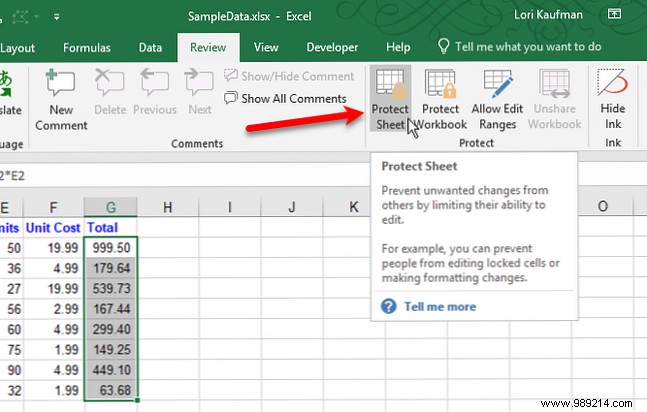
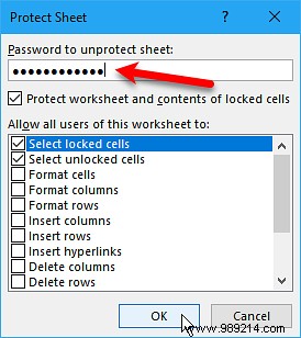
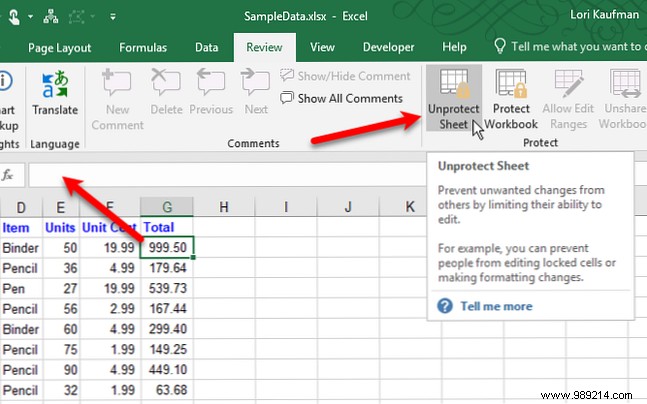
Then Review tab > Protect group > Protect Sheet. Check Protect worksheet and contents of locked cells. Add password (recommended). Adjust permissions like Select locked/unlocked cells.
Formulas hide from the bar; results show unless contents are hidden too. Unhide: Review > Unprotect Sheet (enter password), then uncheck Hidden in Format Cells.
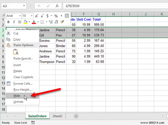
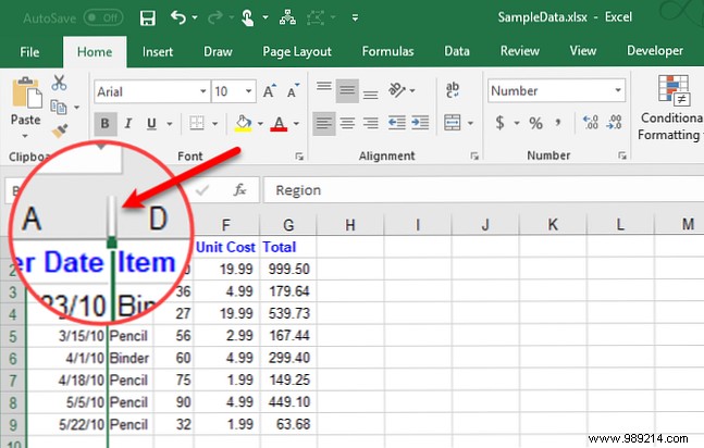
Conceal rows/columns temporarily without deletion. Select consecutive ones, right-click Hide or Ctrl + 9 (rows)/Ctrl + 0 (columns).
Indicators: Double line in headers, thin line in sheet.
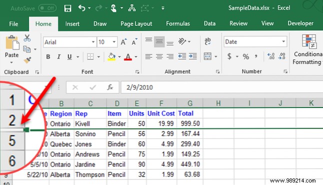
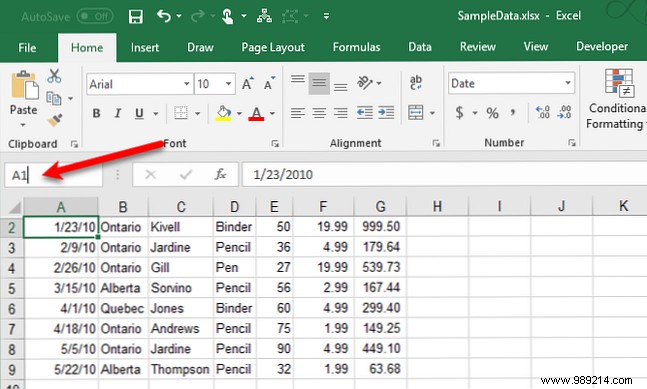
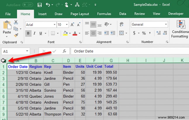
Unhide: Select adjacent rows/columns above/below, right-click Unhide or Ctrl + Shift + 9/0. For row/column A: Name box > A1 > Enter > shortcut.
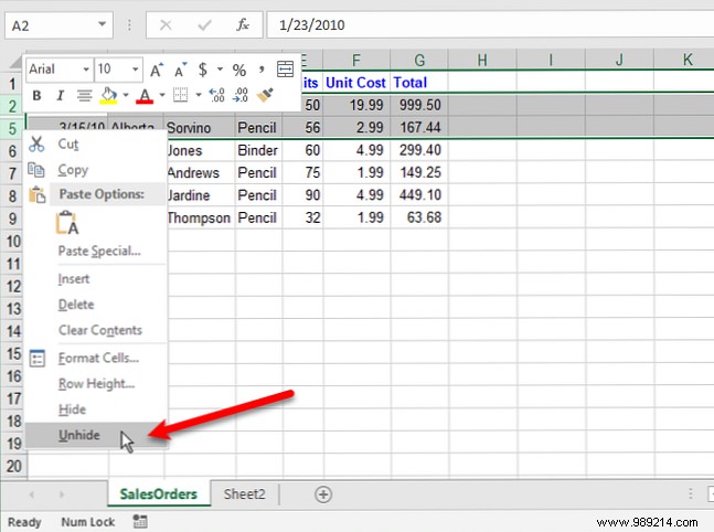
All at once: Select sheet (Ctrl + A), apply unhide shortcuts or right-click headers.
Hiding elements is a core skill for efficient spreadsheets, especially presentations. Input all data, hide what's unnecessary—confidential or auxiliary. Explore our beginner’s Excel guide or row/column hiding tutorial, and 16 essential formulas.